Aggregating partial ranked lists of Escape Room difficulty

TLDR

• Aggregated 1000 partial escape room ranked lists into a single global ranking.
• Compared TrueSkill, GA, and Bradley–Terry (BTL) in a simulator with a known ground-truth ordering.
• Evaluation: Kendall’s τ across 100 runs.
• Most stable: TrueSkill (≈0.90–0.93); GA has a higher ceiling but more variance; the naive BTL version is the least stable.

Motivation

An escape room is an interactive room full of puzzles where the goal is to find all clues and escape in at most 60 minutes. Whether you’re a beginner or a more experienced player, it’s useful to know how difficult a room is. If you’re trying puzzles for the first time and go into a very demanding room, you probably won’t enjoy it much; likewise, if you already have many rooms behind you and choose a room designed for children, you likely won’t enjoy it either.

Conclusion: Everyone wants to go to a room that is right at the edge of their abilities (as with many other things in life). That’s why it would be useful if there was a ranking that includes all rooms that a person can refer to when answering the question “Which room should I visit?”

There are ranking lists on various forums and blogs, but the problem is that they are subjective (one person’s opinion) and they are never complete — they don’t include all rooms in a city or country.

Problem

There is no single ranking that includes all rooms and is formed as a consensus of multiple people.

The goal of this project was to design an algorithm that combines multiple different partial ranked lists into one final ranked list.
We can formalize the problem as aggregation of partial ranked lists: from multiple incomplete lists we need to construct a single list that best reflects the true latent difficulty of each room. This formulation resembles well-known ranking problems in preference theory, but it comes with specific challenges: the data is sparse, each respondent adds subjectivity, not all rooms are visited equally often (so popular and less-known rooms appear in ranked lists at very different rates), and the true ordering is not observed directly.
In theory, finding the optimal aggregated ranking under the Kemeny–Young criterion is proven to be NP-hard. Therefore, as in related areas of combinatorial optimization, we turn to heuristics and metaheuristics that produce good-enough solutions in reasonable time.

Overview of methods used and challenges

I approached the problem from multiple angles: I tried some standard ranking methods, a simpler statistical model, and of course, a genetic algorithm.

A classic (and very widely used) way to estimate strength is the Elo rating system. It was originally designed for chess, but it quickly spread to many other zero-sum games and ranking settings in general. The idea is to assign each task (in our case, each room) a rating, and when a player states that one room is harder than another, the ratings are updated slightly. It is based on the relationship between the expected and the actual outcome. In extreme cases, the largest Elo changes happen when a positive outcome was considered almost certain but a negative outcome occurred, and vice versa. The expected outcome is computed from the rating difference.

Microsoft’s TrueSkill is an extension of Elo designed for more complex environments with multiple players and higher uncertainty in outcomes. While Elo is ideal for 1v1 matches, TrueSkill is built for multiple players (in our case: rooms), which is closer to the nature of this problem. In addition to estimating the mean difficulty of a room, we also track the standard deviation (how uncertain we are), which can be useful for less popular rooms. It also handles contradictory lists better, since different players can have different experiences. This is because it does not follow Luce’s choice axiom, which states that relative selection probabilities for one item versus another in a set are unaffected by the presence or absence of other items in the set. Also, unlike plain Elo, TrueSkill updates take variance (the current uncertainty) into account.

The Bradley–Terry (BTL) pairwise-comparison model is a statistical model that aggregates partial ranked lists based on outcomes of pairwise comparisons. The idea is to model the probability that one element is above another as a function of the difference in their latent values. Concretely, we treat all ranked pairs as observations and learn latent values that best explain all observed pairwise comparisons.

Naturally, since this is an NP-hard problem, I also tried a metaheuristic approach, specifically using a genetic algorithm. A genetic algorithm maintains a population of candidate rankings, crosses and mutates them, and keeps those that fit the original data better. Algorithms like simulated annealing could also work well here. The ordering can be represented as a permutation, the objective as the number of disagreements with the partial ranked lists, and the neighborhood as swapping two elements in the list. This approach would likely be very strong if we had a large number of lists (e.g., global-scale rating), because it scales well with many items and conflicting rankings, but I didn’t use it as the final approach because the defined problem does not have that large a dataset.

Escape rooms bring a few specific issues:

• Sparse data — the same group rarely plays many different rooms (almost always less than half), so the comparison matrix is very sparse.
• Different room popularity — not all rooms are equally popular. If we look at TripAdvisor rating counts, some rooms have thousands of ratings while others have only ~50, a two-orders-of-magnitude difference. This implies some rooms appear in very few ranked lists, making their final position harder to estimate.
• Player bias — a group that enjoys logic puzzles may find a room easier than a group that prefers physical tasks. There are also other factors affecting subjective perception, like sleep, stress, etc.
• Changes over time — skill level is not constant; it grows monotonically with the number of rooms played. This can cause players to rate a room they played earlier in their “career” as harder than an equally demanding room they played later.

Simulator for testing solution quality

Since we don’t have a real ranking list to compare against, I tried to simulate the data collection process as realistically as possible so I could compare different aggregation methods.

The simulator can generate a large number of artificial partial ranked lists that mimic real-world room ratings by players. Each partial ranked list is generated by accounting for room popularity, player subjectivity, and experience level, which influences perceived difficulty.

When generating partial ranked lists, I use a Gaussian distribution to model subjectivity and varying experience. In addition, I use weighted sampling without replacement to simulate room popularity.

The quality of the aggregated ranking is evaluated using Kendall’s τ coefficient against a known ground-truth ordering of rooms. The simulator accepts different aggregation functions, which makes it easy to test and compare various heuristic optimization approaches and machine-learning-based methods.

How a single player’s partial ranking is created in the simulator

1. How many rooms does the player rank?
   For each player, the number of rooms they visited is sampled from a normal distribution with mean 4 and standard deviation 2.5. The result is rounded and clipped to at least 1 and at most the total number of rooms. This reflects the fact that different players visit different numbers of rooms, and that such a count can reasonably be modeled by a normal distribution.
2. Which rooms enter the sample?
   Not all rooms are equally popular. The more popular a room is, the more likely the simulator is to choose it. This replicates “market bias”: attractive or well-marketed rooms will appear more often in players’ partial rankings. We need to account for this in aggregation algorithms, to avoid giving such rooms an unfair advantage in the final ranking.
3. The ideal ordering according to truth
   Once the subset is selected, the simulator first orders it exactly as in the ground-truth list known to the simulator. Subjectivity is injected afterwards, but most players are expected to produce rankings that roughly follow the objective truth.
4. Injecting personal bias
   No player judges perfectly. So the simulator makes one pass through the list and allows each adjacent pair to swap places with some probability. The larger the personal bias, the higher that probability. The result is a short ranking that mostly follows the truth but contains a few local mistakes — just like a real blog post or forum comment.

Such a list is called a partial ranking, because it covers only a subset of rooms and is only approximately in the true order. The simulator repeats the above process, for example, 1000 times. Each time, a new player produces their own partial and biased list. We get a large collection of scattered opinions, similar to a real scenario where reviews accumulate across different sites over months. The aggregation algorithm being tested receives only these partial lists. From them it must create a final ranking of all rooms. When the algorithm finishes and returns that list, the simulator compares it to the ground truth using Kendall’s τ coefficient:

• τ = 1 → perfect match
• τ ≈ 0 → barely better than random guessing
• τ = -1 → the ordering is completely reversed
  

This gives each aggregator a clear score from -1 to 1 that measures its accuracy.

Result

To compare the algorithms, the experiment was repeated 100 times: 1000 partial escape-room difficulty lists were generated, passed to each of the three algorithms, and for every resulting global list the Kendall τ score was measured against the hidden ground-truth ordering.

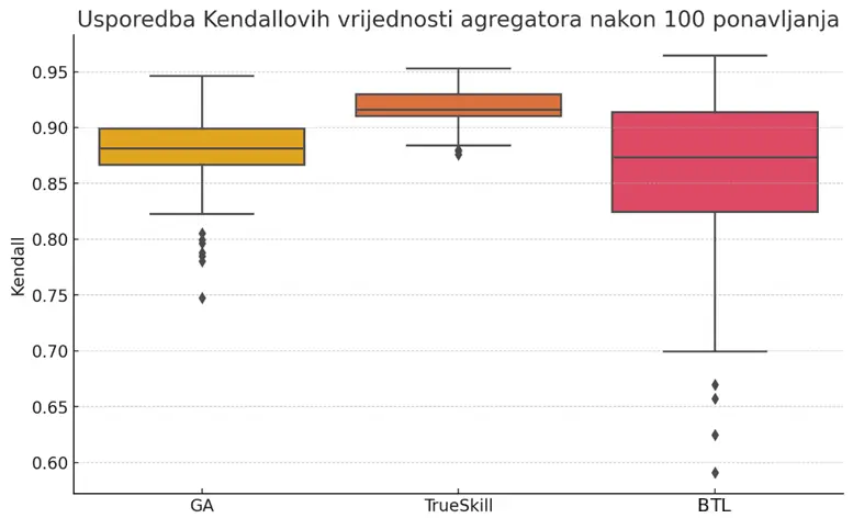
The TrueSkill box is almost flattened: most values are packed into a narrow range between 0.90 and 0.93, and the upper and lower whiskers barely extend beyond that. This suggests the model performs almost equally well in every run. The reason is that TrueSkill assigns a difficulty distribution to each room and updates it with every observation. It keeps uncertainty in view and doesn’t jump wildly when the data isn’t perfect. In practice, that means even when randomness changes the sample of partial lists, the estimates end up almost in the same place.

The genetic algorithm has a median slightly worse than TrueSkill, but its box and whiskers are much taller. Sometimes it reaches peaks around 0.95, and sometimes it drops to 0.82 with occasional outliers around 0.75. This is expected due to the stochastic nature of the heuristic. Most runs head toward the optimal ordering, but occasionally the search gets stuck in a local optimum or loses genetic diversity too early. So GA offers a high ceiling, but it doesn’t guarantee consistently excellent results.

The third column, the BTL logistic model, shows an even wider box and whiskers, with a median around 0.86 and a tail dropping to 0.60. This model performed the worst, as expected, because I used a naive version that assumes pairwise comparisons are homogeneous and independent, which isn’t the case here due to noise from subjectivity. The method is fast and elegant, but it places too much trust in the data not containing systematic bias or gaps. When the same room pair appears rarely, or player bias flips the expected outcome, optimization can easily stall far from the optimum. This model works as a good starting point, but without additional regularization or a larger number of observed pairs it remains the most unstable.

← Back